Mandelbrot: Basic Theory

In this series we’re going to build an app to view the Mandelbrot set. While this is not necessarily something that is likely to be of direct use to the majority of app developers (except for those that have a desire to develop their own Mandelbrot set viewing apps), there are some techniques that we’ll explore along the way that most certainly will be of relevance to many.

I have long had a love of fractals. There is a certain beauty to them both in terms of the mathematics behind them, and the patterns that they create when we graph them. Back when I was first teaching myself how to code, I purchased a book Fractal Programming in C by Roger T. Stevens, and set about writing C apps to render them. I spent many hours tinkering with code to render Koch curves, Peano curves, Hilbert curves, Sierpiński curves, Julia sets, Dragon curves, strange attractors, Lorenz attractors, and many others. But the Mandelbrot set was the first of these that I became aware of, and I have always had a particular fondness for it.

The Mandelbrot set is the set of complex numbers (c) for which repeatedly applying the function fc (z) = z2 + c produces values for which the modulus does not exceed a given value. It this has left you confused, I highly recommend this video which explains all of this is simple terms – there’s no point in me trying to explain it here when there is already a great explanation on YouTube.

To plot the Mandelbrot set, we select a range of complex numbers – we’ll go with the range -2.0 + -1.2i -> 1.0 + 1i. For each pixel in the graph we wish to plot we’ll take the x value as the real component of the complex pair, and the y value as the imaginary component. We’ll then repeatedly apply fc (z) = z2 + c using these values until either the modulus exceeds 2, or we hit an arbitrary iteration limit.

The iteration limit is necessary because there are certain values where we’ll never exceed a modulus of 2 and if we continue iterating indefinitely, we’ll enter an infinite loop. A perfect is example of this is the origin: 0 + 0i which for which the function will always produce 0 + 0i, and no matter how many times we apply the function the the result of the previous iteration, the result will never change. The modulus is essentially the distance of any given value from the origin (which is 0 + 0i itself). So the modulus for this will always be 0. Therefore we need to limit how many times we shall recursively apply the function before determining that the value is within the Mandelbrot set because the modulus has never exceeded 2.

If we plot numbers points which fall within the set in black and those outside it in white we get the following:

Although we can see the overall shape that should be familiar to those who know what plots the Mandelbrot set generally look like, it does not look like some of those colourful plots. Yet. However it does begin to show the complexity of the set boundary.

The key to producing these colourful images is with regard to the points outside of the set. Some complex numbers will have a modulus of 2 even before we begin applying the function, so we know that these will be outside the set. However the ones that are close to the set boundary are the ones that are really interesting, and they can behave in quite unpredictable ways. It is these values and their unpredictability that makes the Mandelbrot set both fascinating and beautiful. Some of these values may require many iterations before they produce a modulus more than 2, and others very close to them may so so in a much lower number of iterations. This variance is visible in the mono render because there are some points much closer to the origin (near the centre of the largest black ‘blob’) which are outside the set yet others that are farther away from the origin which are inside the set. The frilly patterns at the boundary also show this level of variance, as well.

We can apply a colour to the points outside of the set which corresponds to how many iterations were required before we were able to determine that that point was outside the set. The colour scheme that I’m using here uses an HSV colour with the Hue changing depending on how many iterations were required. A low number of iterations will be represented with colours toward the red end of the spectrum, whereas a number of iterations close to the iteration limit will be represented with colours towards the violet end of the spectrum:

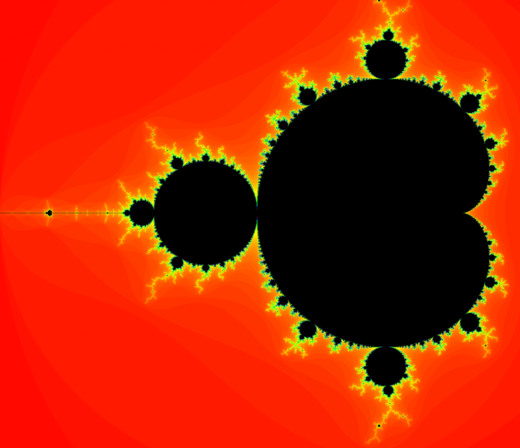
That’s beginning to look much more familiar.

The points far from the origin are red as their modulus exceeds 2 very quickly, but the points close to the set boundary require higher and higher numbers of iterations before their modulus exceeds 2, so we see the colours range in to yellows, then greens, with some blue very close to the boundary.

The iteration limit is quite important here. Too many and it will take a long time to generate the image – all of the points within the set will require us to hit the iteration limit, and many of those just outside the boundary will require us to get close to the limit. However, too few iterations and we’ll lose resolution both in terms of accuracy (we’ll have points that we determine are inside the set which we would actually determine were outside the set with more iterations), and the number of distinct colours which can be represented.

Here is the same rendering but with a much lower iteration limit:

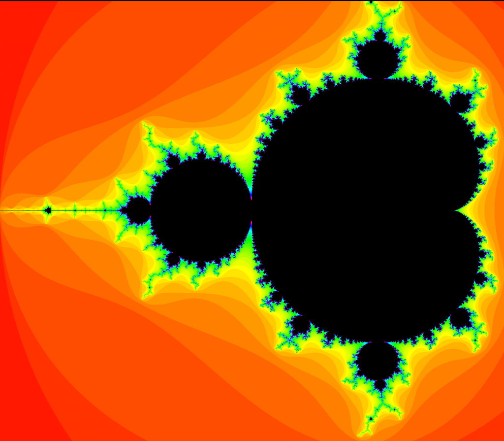
The reduced colour palette is clearly visible in the outer areas, but this version appears to have more blues and purples near the boundary and appears to show more detail. However this is actually an illusion resulting from the reduced resolution and is actually a less accurate rendering. As we progress in the series we’ll see how we can explore the areas close to the boundary,

With the technique that we’ll use to render this the 60 iteration limit renders in around 110ms compared to around 200ms for the 180 iteration limit version.

So there we have the basic theory of what the Mandelbrot is, and the techniques that we’ll use to plot it. Hopefully we’ve also explored a little of why it is interesting and can be quite beautiful – because of the chaotic areas close to the Mandelbrot set boundary.

Apologies that this article has been mainly explaining the theory, however it is necessary to understand a little of how we’ll render things before we dive in to the rendering code. Also, I apologise that there has been nothing Android specific in this article, however the next article will be far more Android-focussed and cover how we can implement the rendering.

There is no source code for this article because we haven’t yet looked at any, but that will follow, I promise!

© 2019, Mark Allison. All rights reserved.

Copyright © 2019 Styling Android. All Rights Reserved.
Information about how to reuse or republish this work may be available at http://blog.stylingandroid.com/license-information.