
Many commercial image processing applications have various effects which are achieved using convolution matrices. These are actually pretty easy to implement on Android and enable us to apply some quite interesting effects to images. In this short series we’ll look a little at the theory behind them, look at some examples of what we can achieve, and, of course, see how we can implement this in our apps.

We’ll start by looking at what image convolution matrices are, how they work, and some of the effects that we can achieve with them.
Fundamentally, convolution matrices are, as the name suggests, and matrix that is applied to an image to transform it in some way. The principle is a near neighbour processing whereby each pixel is transformed using a function of the existing value of that pixel combined with the values of those around it. The simplest form uses a 3×3 matrix.If you imagine the pixel within the image, then think of a 3×3 grid with the target pixel at the centre. If we also consider a 3×3 matrix:

When the matrix is applied to a specific pixel, each of the pixels in the 3×3 grid in the image is multiplied by the value in the corresponding position within the matrix. These values are summed to obtain the new value for the centre pixel of the 3×3 grid.
A simple identity matrix which maps each pixel to the same value (performing no actual processing) would be:

As this is applied, the pixel in question maintains its existing value because the values of surrounding pixels are all multiplied by 0, and the value centre pixel is multiplied by 1. When these are summed, then the value of the centre pixel will be unchanged.
The next simplest matrix to understand is a basic blur:

The overall intensity of the pixel will be unchanged because the sum of all the numbers in the matrix is 1 (or very close to it). In this case, the new value of the centre pixel is an average of all 9 pixels. This could, more accurately, be written as:

We can see the effect if we apply that to an image:

In all of the following examples the top image is unprocessed. I have deliberately chosen quite a low res image here which already looks as though it’s blurred. That is actually deliberate because it makes some of the other transformations we’ll look at easier to see. The bottom image (which has the filter applied, is clearly more blurry though – look at the tip of the paint brush, and the edges of the colours on the palette.
That’s not the only kind of blur that we can do. A gaussian blur uses gaussian weighting for each of the numbers in the matrix:

This is actually more effective if we increase the size of the matrix to 5×5 (which also uses a 5×5 grid surrounding the target pixel:
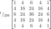
We could expand the box blur to a 5×5 grid in much the same manner:

If we look at the 5×5 gaussian blur we can see that it isn’t noticeably different from the box blur, but it is arguably a more accurate way of performing a blur:

Those with a good memory will remember a previous Styling Android series on blurring images. There is no real reason to use the techniques here over those in the original series unless you specifically require a gaussian or box blur. I have included blur matrices here because I feel that they help in the process of understanding how convolution matrices work. It may seem that we’re limited to blur effects, but if we dig a little deeper there’s actually some other quite cool effects that we can do.
Consider the following matrix:

This is actually going to subtract the values of the surrounding pixels from the target one. The effect of this will vary depending on how similar the target pixel value is to the surrounding ones. If the surrounding values are the same as the target value then we’ll get an output close zero, but if they are generally different then we’ll get a value output. This output image will only contain values where there are differences of the pixel to those surrounding, so it will just show the edges:

While this isn’t necessarily a visually pleasing effect on its own, it shows how convolution matrices can be used to perform processing only on hard edges. Where this can be of more practical use is to sharpen images:

This will effectively lighten and darken pixels around edges, and the overall effect is that the edge is more defined:

This demonstrates the effect, but it’s a little harsh because of the low res image that I used. If we use a higher res image (this is the door to the chamber of secrets that I doing on the Harry Potter Studio Tour a few years back):
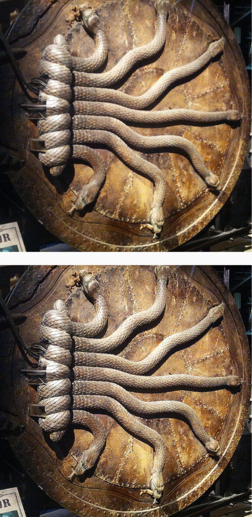
The details like the scales near the hinge are much clearer in the lower image.
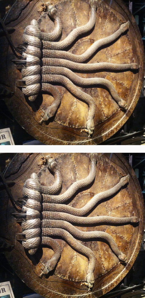
Where this can get even more interesting if if we combine filters by multiplying matrices together. Combining a sharpen filter with a 5×5 gaussian blur we get an unsharp mask filter:

This will improve the perceived definition of an image by applying both a blur and this light / dark edge sharpen that we just looked at. The idea of using a blur to improve definition is a little counter intuitive, but it effective nonetheless. It softens the effect of the sharpen, and makes the edges less harsh, but still well defined:

The effect on the chamber of secrets door is a little more subtle, but it is still a softer effect than the sharpen:
All of the matrices used here were taken from this Wikipedia page, and there are a few other examples there.
While we have only scratched the surface of what is possible using this highly powerful technique, it should be apparent that we can do some quite nice transformations on images. There are a number of Internet resources containing other matrices that can be used – a quick Google search will find them.
In the concluding article in this series we’ll look at how to actually implement this on Android in a really performant manner- it is actually pretty easy.
There is no source code to accompany this article, but it will follow in the next article.
© 2019, Mark Allison. All rights reserved.
Copyright © 2019 Styling Android. All Rights Reserved.
Information about how to reuse or republish this work may be available at http://blog.stylingandroid.com/license-information.